9 Régularisation des moindres carrés : ridge, lasso elastic net

import pandas as pd
import numpy as np
import matplotlib.pyplot as plt
from sklearn.linear_model import Ridge, ElasticNet, Lasso
from sklearn.linear_model import RidgeCV, ElasticNetCV, LassoCV
from sklearn.preprocessing import StandardScaler
from sklearn.linear_model import LinearRegression
from sklearn.pipeline import Pipeline
from sklearn.model_selection import KFold
from patsy import dmatrix

Introduction

Problème du centrage-réduction

Propriétés des estimateurs

Régularisation avec le package scikitlearn

ozone = pd.read_csv("../donnees/ozone.txt", header = 0, sep = ";", index_col=0)
X = ozone.iloc[:,1:10].to_numpy()
y = ozone["O3"].to_numpy()

cr = StandardScaler()
kf = KFold(n_splits=10, shuffle=True, random_state=0)

lassocv = LassoCV(cv=kf)
enetcv = ElasticNetCV(cv=kf)
pipe_lassocv = Pipeline(steps=[("cr", cr), ("lassocv", lassocv)])
pipe_enetcv = Pipeline(steps=[("cr", cr), ("enetcv", enetcv)])

pipe_lassocv.fit(X, y)
pipe_enetcv.fit(X, y)

Pipeline(steps=[('cr', StandardScaler()),
                ('enetcv',
                 ElasticNetCV(cv=KFold(n_splits=10, random_state=0, shuffle=True)))])

In a Jupyter environment, please rerun this cell to show the HTML representation or trust the notebook.
On GitHub, the HTML representation is unable to render, please try loading this page with nbviewer.org.

etape_lassocv = pipe_lassocv.named_steps["lassocv"]
etape_enetcv = pipe_enetcv.named_steps["enetcv"]

alphasridge = etape_lassocv.alphas_ * 100
ridgecv = RidgeCV(cv=kf, alphas=alphasridge)

pipe_ridgecv = Pipeline(steps=[("cr", cr), ("ridgecv", ridgecv)])
pipe_ridgecv.fit(X, y)

Pipeline(steps=[('cr', StandardScaler()),
                ('ridgecv',
                 RidgeCV(alphas=array([1.82214402e+03, 1.69933761e+03, 1.58480794e+03, 1.47799719e+03,
       1.37838513e+03, 1.28548658e+03, 1.19884909e+03, 1.11805068e+03,
       1.04269780e+03, 9.72423459e+02, 9.06885373e+02, 8.45764334e+02,
       7.88762649e+02, 7.35602686e+02, 6.86025527e+02, 6.39789702e+02,
       5.96670018e+02, 5.56456456e+02, 5.18953...
       6.86025527e+00, 6.39789702e+00, 5.96670018e+00, 5.56456456e+00,
       5.18953153e+00, 4.83977447e+00, 4.51358987e+00, 4.20938902e+00,
       3.92569029e+00, 3.66111190e+00, 3.41436521e+00, 3.18424843e+00,
       2.96964074e+00, 2.76949689e+00, 2.58284207e+00, 2.40876716e+00,
       2.24642431e+00, 2.09502283e+00, 1.95382531e+00, 1.82214402e+00]),
                         cv=KFold(n_splits=10, random_state=0, shuffle=True)))])

etape_ridgecv = pipe_ridgecv.named_steps["ridgecv"]

alphas = pipe_lassocv.named_steps["lassocv"].alphas_
coefs_lasso = []; coefs_enet = []; coefs_ridge = []
Xcr = StandardScaler().fit(X).transform(X)
for a in alphas:
    ## lasso
    lasso = Lasso(alpha=a, warm_start=True).fit(Xcr, y)
    coefs_lasso.append(lasso.coef_)
    ## enet
    enet = ElasticNet(alpha=a*2, warm_start=True).fit(Xcr, y)
    coefs_enet.append(enet.coef_)
    ## ridge
    ridge = Ridge(alpha=a*100).fit(Xcr, y)
    coefs_ridge.append(ridge.coef_)
fig, (ax1, ax2, ax3) = plt.subplots(1, 3)
ax1.plot(np.log(alphas), coefs_lasso)
ax1.set_xlabel(r'$\log(\alpha)$')
ax1.set_ylabel('Coefficients')
ax2.plot(np.log(2*alphas), coefs_enet)
ax2.set_xlabel(r'$\log(2\alpha)$')
ax2.set_ylabel('Coefficients')
ax3.plot(np.log(100*alphas), coefs_ridge)
ax3.set_xlabel(r'$\log(100\alpha)$')
ax3.set_ylabel('Coefficients')

Text(0, 0.5, 'Coefficients')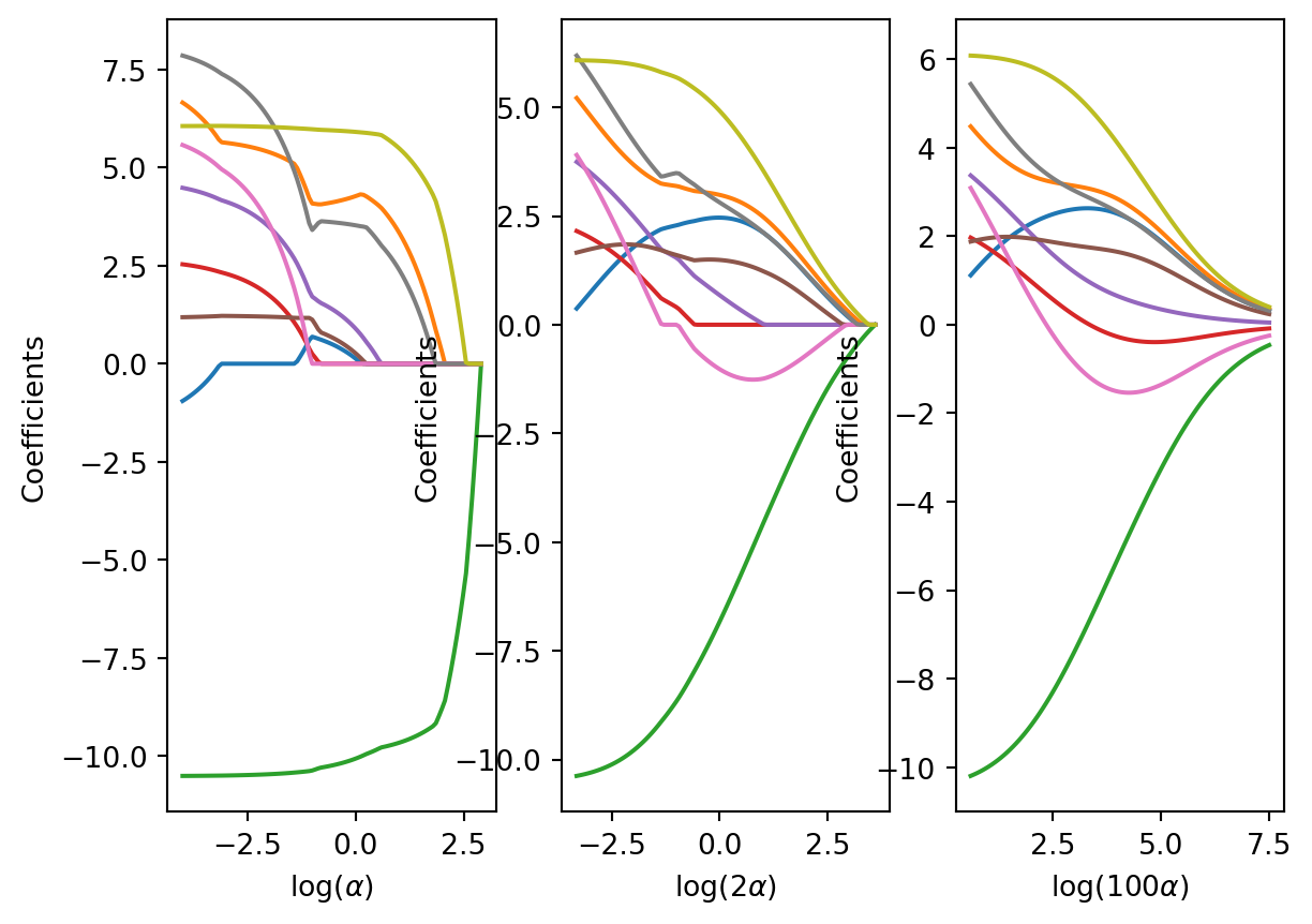

print("Lasso: ", round(etape_lassocv.alpha_,4))
print("ElasticNet: ", round(etape_enetcv.alpha_,4))
print("Ridge: ", round(etape_ridgecv.alpha_,4))

Lasso:  0.7356
ElasticNet:  0.3399
Ridge:  9.0689

ozone = pd.read_csv("../donnees/ozone.txt", header = 0, sep = ";", index_col=0)
Xapp = ozone.iloc[0:45,1:10].to_numpy()
Xnew = ozone.iloc[45:50,1:10].to_numpy()
yapp = np.ravel(ozone.iloc[0:45,:1])
ynew = np.ravel(ozone.iloc[45:50,:1])

kf = KFold(n_splits=10, shuffle=True, random_state=0)
cr = StandardScaler()
lassocv = LassoCV(cv=kf)
pipe_lassocv = Pipeline(steps=[("cr", cr), ("lassocv", lassocv)])
pipe_lassocv.fit(Xapp,yapp)

Pipeline(steps=[('cr', StandardScaler()),
                ('lassocv',
                 LassoCV(cv=KFold(n_splits=10, random_state=0, shuffle=True)))])

pipe_lassocv.predict(Xnew)

array([95.81725767, 63.675633  , 67.49560903, 67.57922292, 89.43629205])

Intégration de variables qualitatives

ozone = pd.read_csv("../donnees/ozone.txt", header=0, sep=";", index_col=0)
ozone["vent"]=ozone["vent"].astype("category")
ozone["nebu"]=ozone["nebu"].astype("category")

kf = KFold(n_splits=10, shuffle=True, random_state=0)
cr = StandardScaler()
lassocv = LassoCV(cv=kf)
enetcv = ElasticNetCV(cv=kf)
pipe_lassocv = Pipeline(steps=[("cr", cr), ("lassocv", lassocv)])

noms = list(ozone.iloc[:, 1:].columns)
formule = "~" + "+".join(noms[0:])
Xq = dmatrix(formule, ozone, return_type="dataframe")
Xapp = Xq.iloc[0:45, 1:].to_numpy()
Xnew = Xq.iloc[45:50, 1:].to_numpy()
yapp = np.ravel(ozone.iloc[0:45,:1])
ynew = np.ravel(ozone.iloc[45:50,:1])

pipe_lassocv.fit(Xapp, yapp)
pipe_lassocv.predict(Xnew).round(2)

array([97.41, 63.72, 66.26, 66.76, 90.23])

formule = "~" + "+".join(noms[0:]) + "+C(vent,Treatment(1))"
Xq = dmatrix(formule,ozone,return_type="dataframe")
Xapp = Xq.iloc[0:45,1:].to_numpy()
Xnew = Xq.iloc[45:50,1:].to_numpy()
yapp = np.ravel(ozone.iloc[0:45,:1])
ynew = np.ravel(ozone.iloc[45:50,:1])
pipe_lassocv.fit(Xapp,yapp)
pipe_lassocv.predict(Xnew).round(2)

array([97.92, 63.63, 65.91, 66.42, 90.29])

formule = "~" + "+".join(noms[0:-2]) + \
"+ C(nebu, Sum) + C(vent, Sum)"
Xq = dmatrix(formule,ozone,return_type="dataframe")
Xapp = Xq.iloc[0:45,1:].to_numpy()
Xnew = Xq.iloc[45:50,1:].to_numpy()
yapp = np.ravel(ozone.iloc[0:45,:1])
ynew = np.ravel(ozone.iloc[45:50,:1])
pipe_lassocv.fit(Xapp,yapp)
pipe_lassocv.predict(Xnew).round(2)

array([99.49, 63.82, 65.65, 66.18, 90.31])

Retour au sommet