import numpy as np; import pandas as pd
import matplotlib
import matplotlib.pyplot as plt
import scipy.stats as stats
import statsmodels.formula.api as smf
import statsmodels.api as sm6 Inférence dans le modèle gaussien
ozone = pd.read_csv("../donnees/ozone.txt", header=0, sep=";")
mod3 = smf.ols("O3 ~ T12+Vx+Ne12", data=ozone).fit()
print(mod3.conf_int(alpha=0.05))
0 1
Intercept 57.158415 111.936250
T12 0.313811 2.316281
Vx 0.149186 0.823705
Ne12 -6.960609 -2.826137mod3.summary()
ICparams=mod3.conf_int(alpha=0.05)
mod3.params
stats.t.ppf(0.95, mod3.df_resid)
ICparams=mod3.conf_int(alpha=0.025)
def ellipse(m, ij, alpha=0.05, npoints=500):
import numpy as np
from scipy.stats import f
hatSigma = m.cov_params().iloc[ij,ij]
valpr,vectpr = np.linalg.eig(hatSigma)
hatSigmademi = vectpr @ np.diag(np.sqrt(valpr))
theta = np.linspace(0, 2 * np.pi, npoints)
rho = (2 * f.isf(alpha, 2, m.nobs - 2))**0.5
XX = np.array([rho * np.cos(theta), rho * np.sin(theta)])
ZZ = np.add((hatSigmademi @ XX).T, m.params.iloc[ij].to_numpy())
return ZZ
fig = plt.figure()
fig, axs = plt.subplots(3, 2,figsize=(8, 8))
ic = 0
il = 0
for i in range(0,3):
for j in range(i+1,4):
coord = ellipse(mod3, [i, j])
axs[il,ic].fill(coord[:,0], coord[:,1], fc='lightgrey', ec='k', lw=1)
axs[il,ic].plot(mod3.params.iloc[i], mod3.params.iloc[j], "+")
r = matplotlib.patches.Rectangle(ICparams.iloc[[i, j], 0], ICparams.diff(axis=1).iloc[i, 1], ICparams.diff(axis=1).iloc[j, 1], fill=False)
axs[il,ic].add_artist(r)
if ic==0:
ic = 1
else:
ic = 0
il += 1
fig.tight_layout() <Figure size 672x480 with 0 Axes>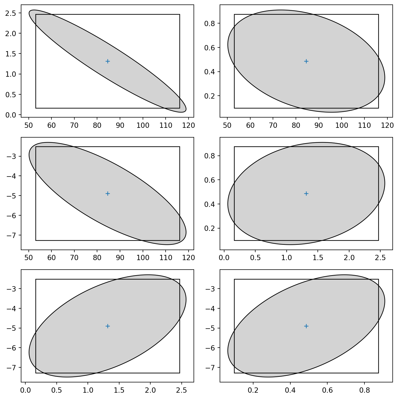
#print(mod3.scale*mod3.df_resid/scipy.stats.chi2.ppf(0.975,mod3.df_resid))
#print(mod3.scale*mod3.df_resid/scipy.stats.chi2.ppf(0.025,mod3.df_resid))
Exemple 1 : la concentration en ozone
mod3 = smf.ols("O3 ~ T12 + Vx + Ne12",data=ozone).fit()
mod3.summary()| Dep. Variable: | O3 | R-squared: | 0.682 |
| Model: | OLS | Adj. R-squared: | 0.661 |
| Method: | Least Squares | F-statistic: | 32.87 |
| Date: | Thu, 27 Mar 2025 | Prob (F-statistic): | 1.66e-11 |
| Time: | 16:23:25 | Log-Likelihood: | -200.50 |
| No. Observations: | 50 | AIC: | 409.0 |
| Df Residuals: | 46 | BIC: | 416.7 |
| Df Model: | 3 | ||
| Covariance Type: | nonrobust |
| coef | std err | t | P>|t| | [0.025 | 0.975] | |
| Intercept | 84.5473 | 13.607 | 6.214 | 0.000 | 57.158 | 111.936 |
| T12 | 1.3150 | 0.497 | 2.644 | 0.011 | 0.314 | 2.316 |
| Vx | 0.4864 | 0.168 | 2.903 | 0.006 | 0.149 | 0.824 |
| Ne12 | -4.8934 | 1.027 | -4.765 | 0.000 | -6.961 | -2.826 |
| Omnibus: | 0.211 | Durbin-Watson: | 1.758 |
| Prob(Omnibus): | 0.900 | Jarque-Bera (JB): | 0.411 |
| Skew: | -0.050 | Prob(JB): | 0.814 |
| Kurtosis: | 2.567 | Cond. No. | 148. |
Notes:
[1] Standard Errors assume that the covariance matrix of the errors is correctly specified.
mod3.conf_int(alpha=0.05)| 0 | 1 | |
|---|---|---|
| Intercept | 57.158415 | 111.936250 |
| T12 | 0.313811 | 2.316281 |
| Vx | 0.149186 | 0.823705 |
| Ne12 | -6.960609 | -2.826137 |
mod2 = smf.ols("O3 ~ T12 + Vx",data=ozone).fit()
round(sm.stats.anova_lm(mod2,mod3),3)| df_resid | ssr | df_diff | ss_diff | F | Pr(>F) | |
|---|---|---|---|---|---|---|
| 0 | 47.0 | 13299.399 | 0.0 | NaN | NaN | NaN |
| 1 | 46.0 | 8904.622 | 1.0 | 4394.777 | 22.703 | 0.0 |
Exemple 2 : la hauteur des eucalyptus
eucalyptus = pd.read_csv("../donnees/eucalyptus.txt",header=0,sep=";")
regS = smf.ols('ht~circ', data=eucalyptus).fit()
regM = smf.ols('ht~circ +  np.sqrt(circ)', data=eucalyptus).fit()
round(sm.stats.anova_lm(regS,regM),3)| df_resid | ssr | df_diff | ss_diff | F | Pr(>F) | |
|---|---|---|---|---|---|---|
| 0 | 1427.0 | 2052.084 | 0.0 | NaN | NaN | NaN |
| 1 | 1426.0 | 1840.656 | 1.0 | 211.428 | 163.798 | 0.0 |
regM.summary()| Dep. Variable: | ht | R-squared: | 0.792 |
| Model: | OLS | Adj. R-squared: | 0.792 |
| Method: | Least Squares | F-statistic: | 2718. |
| Date: | Thu, 27 Mar 2025 | Prob (F-statistic): | 0.00 |
| Time: | 16:23:25 | Log-Likelihood: | -2208.5 |
| No. Observations: | 1429 | AIC: | 4423. |
| Df Residuals: | 1426 | BIC: | 4439. |
| Df Model: | 2 | ||
| Covariance Type: | nonrobust |
| coef | std err | t | P>|t| | [0.025 | 0.975] | |
| Intercept | -24.3520 | 2.614 | -9.314 | 0.000 | -29.481 | -19.223 |
| circ | -0.4829 | 0.058 | -8.336 | 0.000 | -0.597 | -0.369 |
| np.sqrt(circ) | 9.9869 | 0.780 | 12.798 | 0.000 | 8.456 | 11.518 |
| Omnibus: | 3.015 | Durbin-Watson: | 0.947 |
| Prob(Omnibus): | 0.221 | Jarque-Bera (JB): | 2.897 |
| Skew: | -0.097 | Prob(JB): | 0.235 |
| Kurtosis: | 3.103 | Cond. No. | 4.41e+03 |
Notes:
[1] Standard Errors assume that the covariance matrix of the errors is correctly specified.
[2] The condition number is large, 4.41e+03. This might indicate that there are
strong multicollinearity or other numerical problems.
grille = pd.DataFrame({'circ' : np.linspace(eucalyptus["circ"].min(),eucalyptus["circ"].max(),100)})
calculprev = regM.get_prediction(grille)
prev = calculprev.predicted_mean
ICdte = calculprev.conf_int(obs=False, alpha=0.05)
ICpre = calculprev.conf_int(obs=True, alpha=0.05)
fig = plt.figure()
plt.plot(eucalyptus["circ"], eucalyptus["ht"], '+k')
plt.ylabel('ht') ; plt.xlabel('circ')
plt.plot(grille['circ'],  prev, '-', label="E(Y)", lw=1)
lesic, = plt.plot(grille['circ'], ICdte[:,0], 'r--', label=r"IC $\mathbb{E}(Y)$",lw=1)
plt.plot(grille['circ'], ICdte[:, 1], 'r--', lw=1)
lesic2, = plt.plot(grille['circ'], ICpre[:, 0], 'g:', label=r"IC $Y$",lw=1)
plt.plot(grille['circ'], ICpre[:, 1],'g:', lw=1)
plt.legend(handles=[lesic, lesic2], loc='lower right')
fig.tight_layout()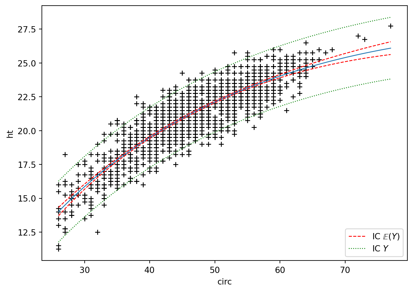
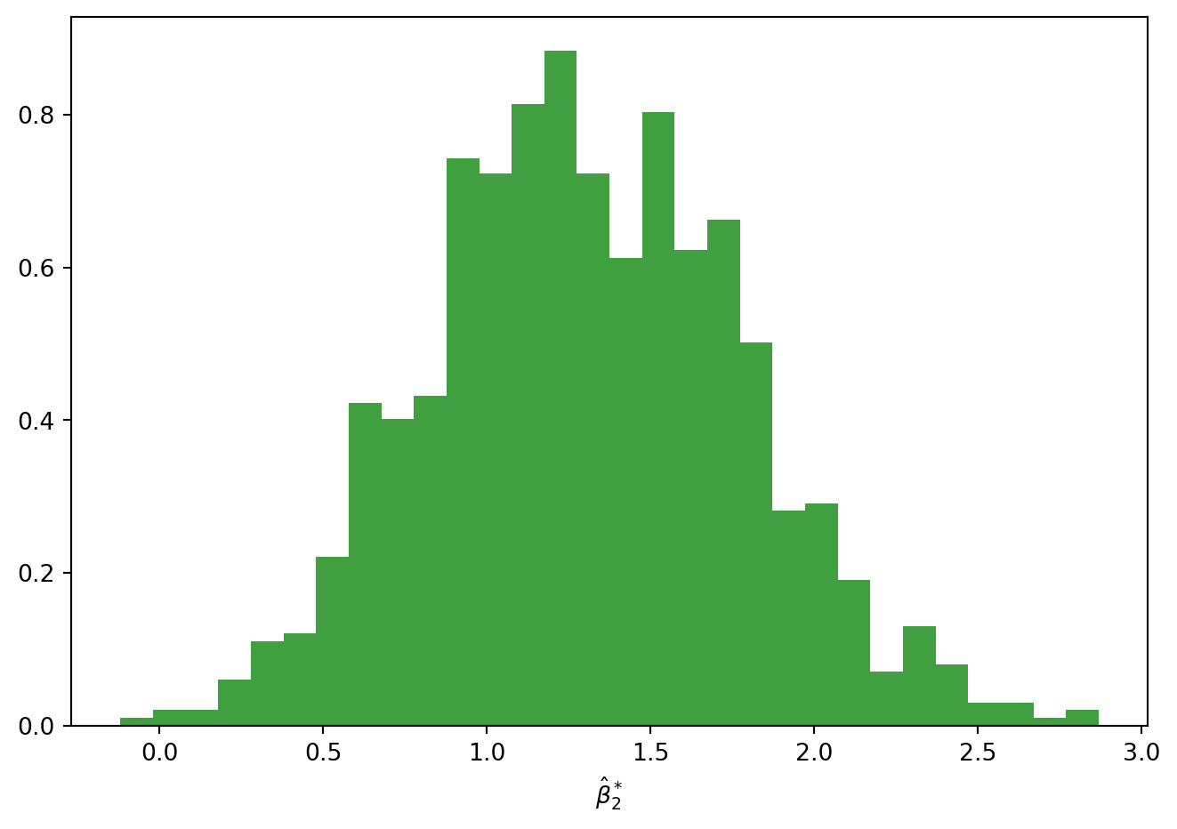
Intervlle de confiance : boostrap
mod3 = smf.ols("O3 ~ 1 + T12 + Vx + Ne12", data = ozone).fit()

mod3.params
mod3.scale
residus3 = mod3.resid
ychap = mod3.fittedvalues
n = residus3.shape[0]

B = 1000
COEFF = np.zeros((B, 4))
rng = np.random.default_rng(seed=1234)
ozoneetoile = ozone[["O3", "T12" , "Vx",  "Ne12"]].copy()
for  b in range(B):
    resetoile = residus3[rng.integers(n, size=n)]
    O3etoile = np.add(ychap.values ,resetoile.values)
    ozoneetoile.loc[:,"O3"] = O3etoile
    regboot = smf.ols("O3 ~ 1+ T12 + Vx + Ne12", data=ozoneetoile).fit()
    COEFF[b] = regboot.params.values


print(np.quantile(COEFF,[0.025, 0.975],axis=0))

fig = plt.figure()
n, bins, patches = plt.hist(COEFF[:,1], 30, density=True, facecolor='g', alpha=0.75)
plt.xlabel(r'$\hat \beta_{2}^*$')
fig.tight_layout()
[[ 58.65115402 0.44272441 0.18933792 -6.84767267]
[108.56181699 2.31524345 0.80828089 -2.7953567 ]]