1 Régression simple

La concentration en ozone

import pandas as pd
import numpy as np
import matplotlib.pyplot as plt
import statsmodels.formula.api as smf

ozone = pd.read_csv("../donnees/ozone_simple.txt", header=0, sep=";")
plt.plot(ozone.T12, ozone.O3, '.k')
plt.ylabel('O3')
plt.xlabel('T12')
plt.show()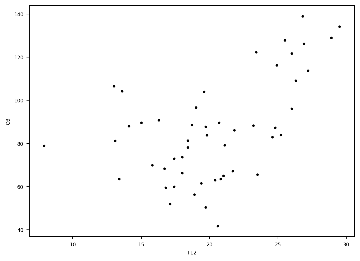

reg = smf.ols('O3 ~ T12', data=ozone).fit()
reg.summary()

OLS Regression Results
Dep. Variable:	O3	R-squared:	0.279
Model:	OLS	Adj. R-squared:	0.264
Method:	Least Squares	F-statistic:	18.58
Date:	Fri, 31 Jan 2025	Prob (F-statistic):	8.04e-05
Time:	15:41:21	Log-Likelihood:	-220.96
No. Observations:	50	AIC:	445.9
Df Residuals:	48	BIC:	449.7
Df Model:	1
Covariance Type:	nonrobust

	coef	std err	t	P>\|t\|	[0.025	0.975]
Intercept	31.4150	13.058	2.406	0.020	5.159	57.671
T12	2.7010	0.627	4.311	0.000	1.441	3.961

Omnibus:	2.252	Durbin-Watson:	1.461
Prob(Omnibus):	0.324	Jarque-Bera (JB):	1.348
Skew:	0.026	Prob(JB):	0.510
Kurtosis:	2.197	Cond. No.	94.1

Notes:
[1] Standard Errors assume that the covariance matrix of the errors is correctly specified.

grille = pd.DataFrame({'T12': np.linspace(ozone.T12.min(), ozone.T12.max(), 100)})
calculprev = reg.get_prediction(grille)
ICdte = calculprev.conf_int(obs=False, alpha=0.05)
prev = calculprev.predicted_mean
ICprev = calculprev.conf_int(obs=True, alpha=0.05)

plt.plot(ozone.T12, ozone.O3, '.k')
plt.ylabel('O3')
plt.xlabel('T12')
plt.plot(grille.T12,  prev, '-', lw=1, label="E(Y)")
lesic, = plt.plot(grille.T12, ICdte[:, 0], 'r--', label=r"IC $\mathbb{E}(Y)$", lw=1)
plt.plot(grille.T12, ICdte[:, 1], 'r--', lw=1)
plt.legend(handles=[lesic,], loc='lower right')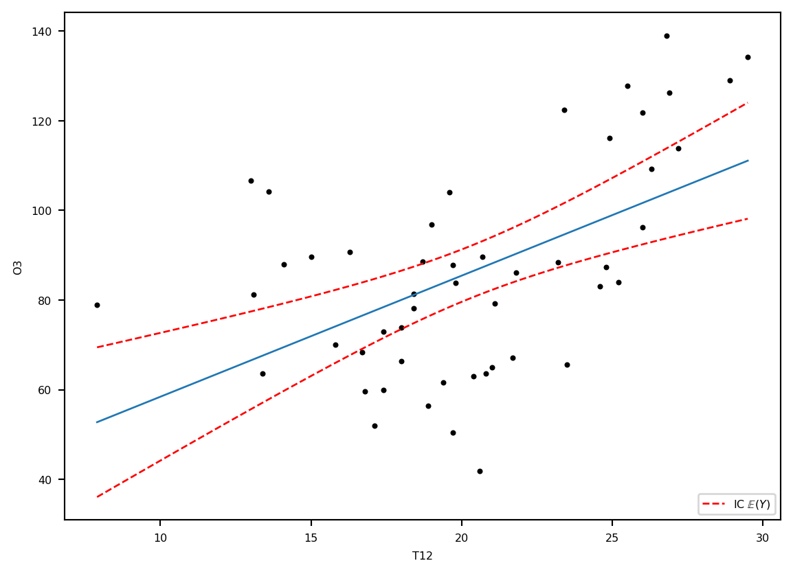

plt.plot(ozone.T12, ozone.O3, '.k')
plt.ylabel('O3') ; plt.xlabel('T12')
plt.plot(grille.T12,  prev, '-', lw=1, label="E(Y)")
lesic, = plt.plot(grille.T12, ICdte[:, 0], 'r--', label=r"IC $\mathbb{E}(Y)$", lw=1)
plt.plot(grille.T12, ICdte[:, 1],'r--', lw=1)

lesic2, = plt.plot(grille.T12, ICprev[:, 0], 'g:', label=r"IC $Y$", lw=1)
plt.plot(grille.T12, ICprev[:, 1],'g:', lw=1)
plt.legend(handles=[lesic, lesic2], loc='lower right')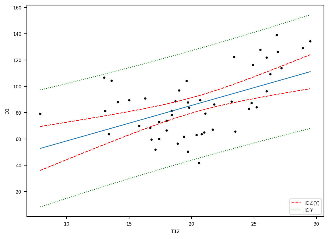

ICparams = reg.conf_int(alpha=0.05)
round(ICparams, 3)

	0	1
Intercept	5.159	57.671
T12	1.441	3.961

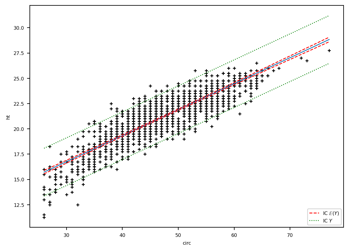
La hauteur des eucalyptus

eucalyptus = pd.read_csv("../donnees/eucalyptus.txt", header=0, sep=";")
plt.plot(eucalyptus.circ, eucalyptus.ht, '+k')
plt.ylabel('ht')
plt.xlabel('circ')
plt.show()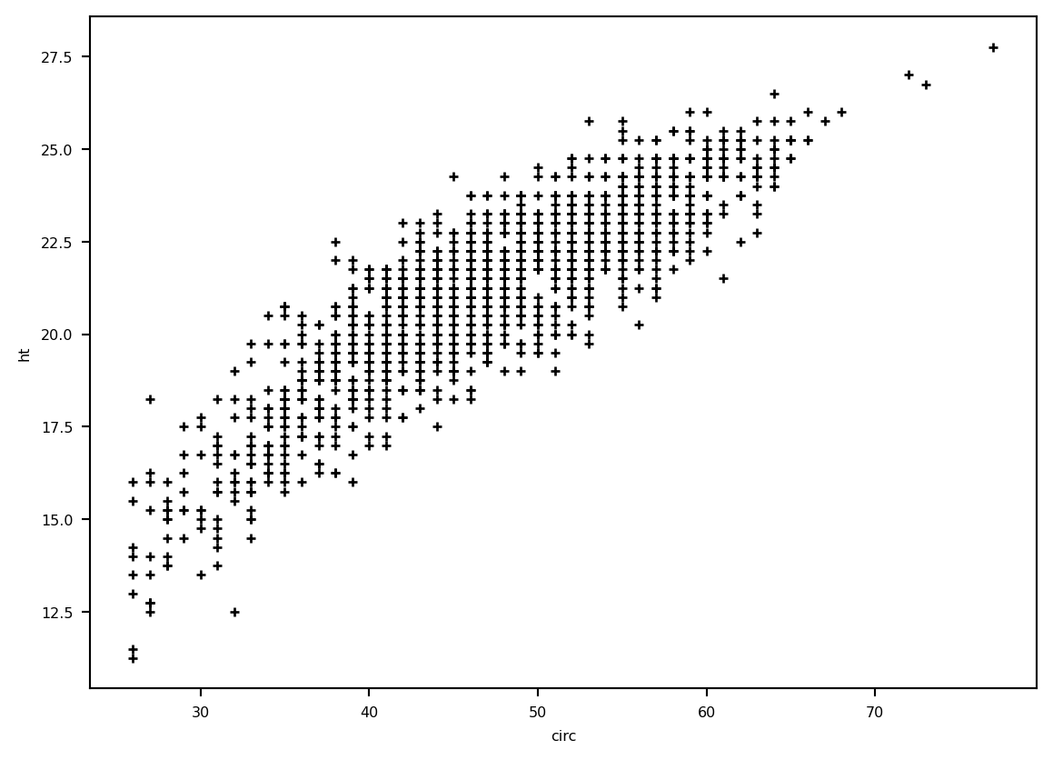

reg = smf.ols('ht ~ circ', data=eucalyptus).fit()
reg.summary()

OLS Regression Results
Dep. Variable:	ht	R-squared:	0.768
Model:	OLS	Adj. R-squared:	0.768
Method:	Least Squares	F-statistic:	4732.
Date:	Fri, 31 Jan 2025	Prob (F-statistic):	0.00
Time:	15:41:22	Log-Likelihood:	-2286.2
No. Observations:	1429	AIC:	4576.
Df Residuals:	1427	BIC:	4587.
Df Model:	1
Covariance Type:	nonrobust

	coef	std err	t	P>\|t\|	[0.025	0.975]
Intercept	9.0375	0.180	50.264	0.000	8.685	9.390
circ	0.2571	0.004	68.792	0.000	0.250	0.264

Omnibus:	7.943	Durbin-Watson:	1.067
Prob(Omnibus):	0.019	Jarque-Bera (JB):	8.015
Skew:	-0.156	Prob(JB):	0.0182
Kurtosis:	3.193	Cond. No.	273.

Notes:
[1] Standard Errors assume that the covariance matrix of the errors is correctly specified.

grille = pd.DataFrame({'circ' : np.linspace(eucalyptus.circ.min(), eucalyptus.circ.max(), 100)})
calculprev = reg.get_prediction(grille)
ICdte = calculprev.conf_int(obs=False, alpha=0.05)
ICprev = calculprev.conf_int(obs=True, alpha=0.05)
prev = calculprev.predicted_mean

plt.plot(eucalyptus.circ, eucalyptus.ht, '+k')
plt.ylabel('ht') ; plt.xlabel('circ')
plt.plot(grille.circ,  prev, '-', label="E(Y)", lw=1)
lesic, = plt.plot(grille.circ, ICdte[:, 0], 'r--', label=r"IC $\mathbb{E}(Y)$", lw=1)
plt.plot(grille.circ, ICdte[:, 1], 'r--', lw=1)
plt.legend(handles=[lesic], loc='lower right')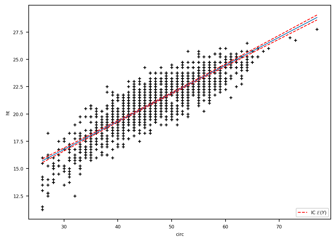

plt.plot(eucalyptus.circ, eucalyptus.ht, '+k')
plt.ylabel('ht') ; plt.xlabel('circ')
plt.plot(grille.circ,  prev, '-', label="E(Y)", lw=1)
lesic, = plt.plot(grille.circ, ICdte[:, 0], 'r--', label=r"IC $\mathbb{E}(Y)$", lw=1)
plt.plot(grille.circ, ICdte[:, 1], 'r--', lw=1)
lesic2, = plt.plot(grille.circ, ICprev[:, 0], 'g:', label=r"IC $Y$", lw=1)
plt.plot(grille.circ, ICprev[:, 1],'g:', lw=1)
plt.legend(handles=[lesic, lesic2], loc='lower right')

Retour au sommet