import pandas as pd
import numpy as np
import matplotlib.pyplot as plt
from mpl_toolkits.mplot3d import Axes3D
import statsmodels.api as sm
import statsmodels.formula.api as smf2 La régression linéaire multiple
La concentration en ozone
ozone = pd.read_csv("../donnees/ozone.txt", header=0, sep=";")fig = plt.figure()
ax = fig.add_subplot(111, projection='3d')
ax.scatter(ozone.T12, ozone.Vx,ozone.O3)
ax.set_xlabel('T12') ; ax.set_ylabel('Vx') ; ax.set_zlabel('O3')
fig.tight_layout()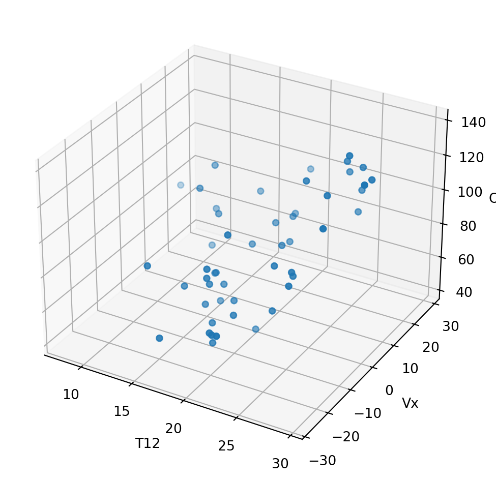
reg = smf.ols('O3 ~ T12+Vx', data=ozone).fit()
reg.summary()| Dep. Variable: | O3 | R-squared: | 0.525 |
| Model: | OLS | Adj. R-squared: | 0.505 |
| Method: | Least Squares | F-statistic: | 25.96 |
| Date: | Fri, 31 Jan 2025 | Prob (F-statistic): | 2.54e-08 |
| Time: | 17:30:04 | Log-Likelihood: | -210.53 |
| No. Observations: | 50 | AIC: | 427.1 |
| Df Residuals: | 47 | BIC: | 432.8 |
| Df Model: | 2 | ||
| Covariance Type: | nonrobust |
| coef | std err | t | P>|t| | [0.025 | 0.975] | |
| Intercept | 35.4530 | 10.745 | 3.300 | 0.002 | 13.838 | 57.068 |
| T12 | 2.5380 | 0.515 | 4.927 | 0.000 | 1.502 | 3.574 |
| Vx | 0.8736 | 0.177 | 4.931 | 0.000 | 0.517 | 1.230 |
| Omnibus: | 0.280 | Durbin-Watson: | 1.678 |
| Prob(Omnibus): | 0.869 | Jarque-Bera (JB): | 0.331 |
| Skew: | 0.165 | Prob(JB): | 0.848 |
| Kurtosis: | 2.777 | Cond. No. | 94.4 |
Notes:
[1] Standard Errors assume that the covariance matrix of the errors is correctly specified.
La hauteur des eucalyptus
eucalyptus = pd.read_csv("../donnees/eucalyptus.txt",header=0,sep=";")
fig = plt.figure()
plt.plot(eucalyptus.circ, eucalyptus.ht, '+k')
plt.ylabel('ht') ; plt.xlabel('circ')
fig.tight_layout()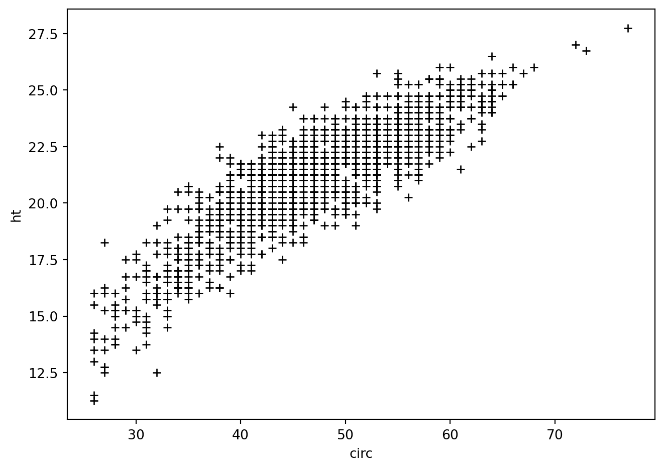
reg = smf.ols('ht ~ circ+np.sqrt(circ)', data=eucalyptus).fit()
reg.summary()| Dep. Variable: | ht | R-squared: | 0.792 |
| Model: | OLS | Adj. R-squared: | 0.792 |
| Method: | Least Squares | F-statistic: | 2718. |
| Date: | Fri, 31 Jan 2025 | Prob (F-statistic): | 0.00 |
| Time: | 17:30:04 | Log-Likelihood: | -2208.5 |
| No. Observations: | 1429 | AIC: | 4423. |
| Df Residuals: | 1426 | BIC: | 4439. |
| Df Model: | 2 | ||
| Covariance Type: | nonrobust |
| coef | std err | t | P>|t| | [0.025 | 0.975] | |
| Intercept | -24.3520 | 2.614 | -9.314 | 0.000 | -29.481 | -19.223 |
| circ | -0.4829 | 0.058 | -8.336 | 0.000 | -0.597 | -0.369 |
| np.sqrt(circ) | 9.9869 | 0.780 | 12.798 | 0.000 | 8.456 | 11.518 |
| Omnibus: | 3.015 | Durbin-Watson: | 0.947 |
| Prob(Omnibus): | 0.221 | Jarque-Bera (JB): | 2.897 |
| Skew: | -0.097 | Prob(JB): | 0.235 |
| Kurtosis: | 3.103 | Cond. No. | 4.41e+03 |
Notes:
[1] Standard Errors assume that the covariance matrix of the errors is correctly specified.
[2] The condition number is large, 4.41e+03. This might indicate that there are
strong multicollinearity or other numerical problems.
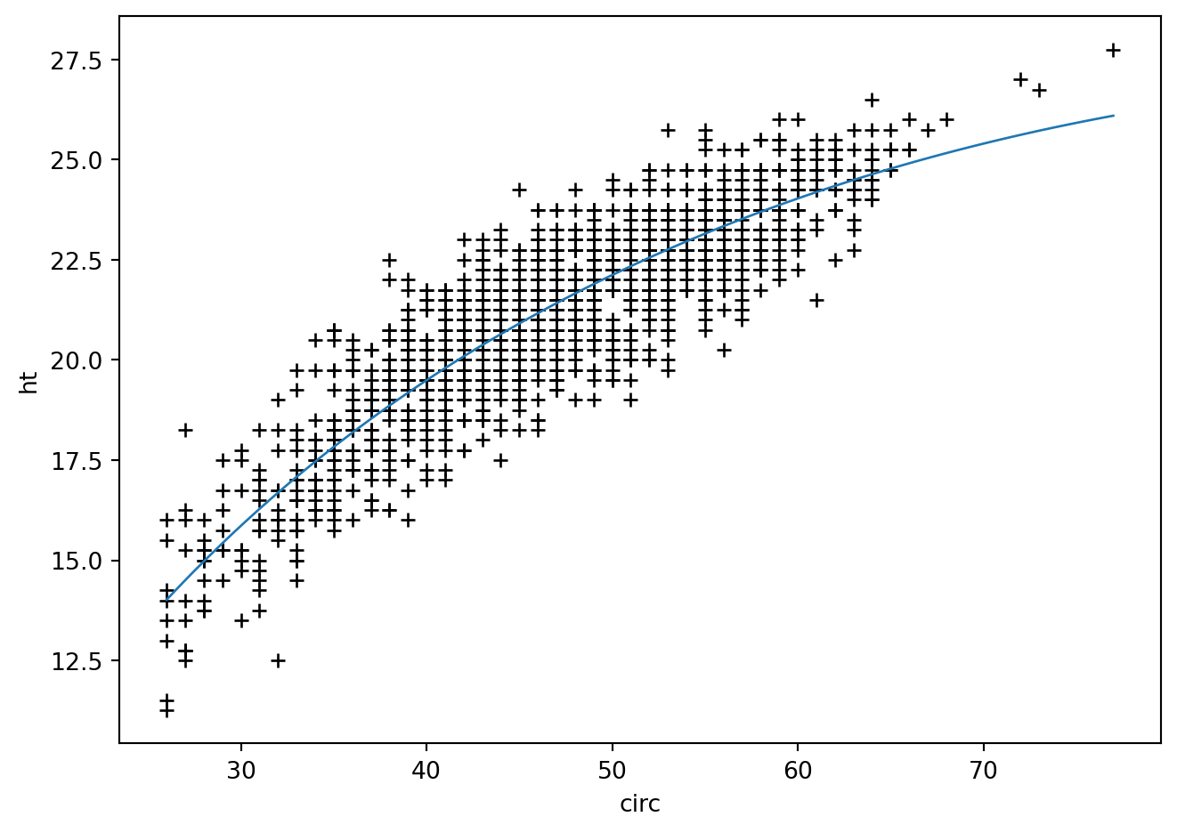
grille = pd.DataFrame({'circ' : np.linspace(eucalyptus.circ.min(), \
                            eucalyptus.circ.max(),100)})
calculprev = reg.get_prediction(grille)
prev = calculprev.predicted_mean

fig = plt.figure()
plt.plot(eucalyptus.circ, eucalyptus.ht, '+k')
plt.ylabel('ht') ; plt.xlabel('circ')
plt.plot(grille.circ, prev, '-', lw=1)
fig.tight_layout()