7 pythonVariables qualitatives : ANCOVA et ANOVA

import pandas as pd; import numpy as np
import matplotlib.pyplot as plt
import matplotlib.cm as cm
import seaborn as sns
import statsmodels.api as sm
import statsmodels.formula.api as smf
from statsmodels.graphics import regressionplots
from statsmodels.graphics.api import interaction_plot
from patsy import dmatrix, ContrastMatrix

fig = plt.figure()
eucalypt = pd.read_csv("../donnees/eucalyptus.txt", header = 0, sep = ";")
eucalypt["bloc"] = eucalypt["bloc"].astype("category")
sns.scatterplot(data=eucalypt, x="circ", y="ht", hue="bloc",style='bloc')
fig.tight_layout()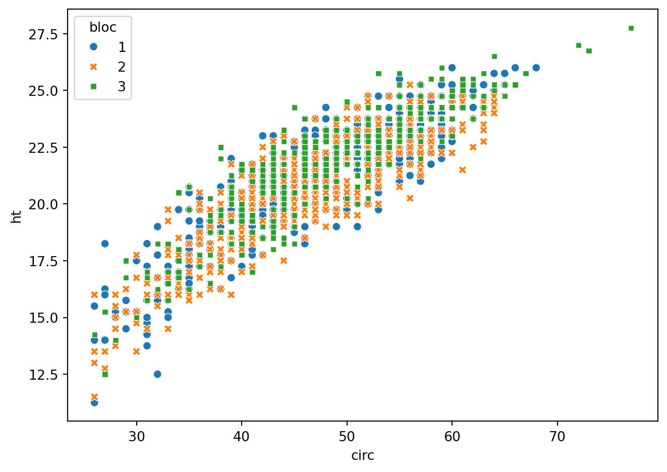

La concentration en ozone

ozone = pd.read_csv("../donnees/ozone.txt", header = 0, sep = ";")
ozone["vent"]=ozone["vent"].astype("category")


niveau = ozone["vent"].cat.categories
cc = cm.Set1(range(niveau.size))
mm = ["o","*","8","s"]
fig, ax = plt.subplots()
for i, val in enumerate(niveau):
    print(val)
    reg = smf.ols("O3 ~ 1 + T12",data=ozone.loc[ozone["vent"]==val]).fit()
    plt.scatter(ozone.loc[ozone["vent"]==val,"T12"],ozone.loc[ozone["vent"]==val,"O3"],
                color=cc[i],label=val, marker=mm[i])
    regressionplots.abline_plot(model_results=reg, ax=ax, color=cc[i])

plt.legend()
fig.tight_layout()

EST
NORD
OUEST
SUD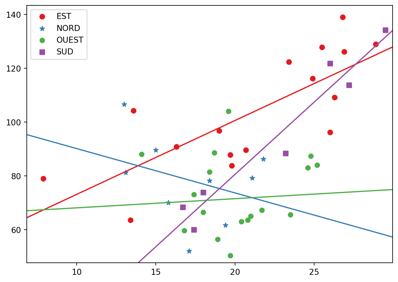

mod1b = smf.ols('O3 ~ -1 + vent + T12:vent', data = ozone).fit()
mod1b.summary()

OLS Regression Results
Dep. Variable:	O3	R-squared:	0.675
Model:	OLS	Adj. R-squared:	0.621
Method:	Least Squares	F-statistic:	12.48
Date:	Thu, 27 Mar 2025	Prob (F-statistic):	1.61e-08
Time:	16:23:49	Log-Likelihood:	-201.01
No. Observations:	50	AIC:	418.0
Df Residuals:	42	BIC:	433.3
Df Model:	7
Covariance Type:	nonrobust

	coef	std err	t	P>\|t\|	[0.025	0.975]
vent[EST]	45.6090	13.934	3.273	0.002	17.488	73.730
vent[NORD]	106.6345	28.034	3.804	0.000	50.059	163.209
vent[OUEST]	64.6840	24.621	2.627	0.012	14.997	114.371
vent[SUD]	-27.0602	26.539	-1.020	0.314	-80.618	26.498
T12:vent[EST]	2.7480	0.634	4.333	0.000	1.468	4.028
T12:vent[NORD]	-1.6491	1.606	-1.027	0.310	-4.890	1.592
T12:vent[OUEST]	0.3407	1.205	0.283	0.779	-2.091	2.772
T12:vent[SUD]	5.3786	1.150	4.678	0.000	3.058	7.699

Omnibus:	0.276	Durbin-Watson:	1.561
Prob(Omnibus):	0.871	Jarque-Bera (JB):	0.465
Skew:	0.007	Prob(JB):	0.793
Kurtosis:	2.528	Cond. No.	168.

Notes:
[1] Standard Errors assume that the covariance matrix of the errors is correctly specified.

mod1 =smf.ols('O3 ~ vent + T12:vent', data = ozone).fit()
mod1.summary()

OLS Regression Results
Dep. Variable:	O3	R-squared:	0.675
Model:	OLS	Adj. R-squared:	0.621
Method:	Least Squares	F-statistic:	12.48
Date:	Thu, 27 Mar 2025	Prob (F-statistic):	1.61e-08
Time:	16:23:49	Log-Likelihood:	-201.01
No. Observations:	50	AIC:	418.0
Df Residuals:	42	BIC:	433.3
Df Model:	7
Covariance Type:	nonrobust

	coef	std err	t	P>\|t\|	[0.025	0.975]
Intercept	45.6090	13.934	3.273	0.002	17.488	73.730
vent[T.NORD]	61.0255	31.306	1.949	0.058	-2.153	124.204
vent[T.OUEST]	19.0751	28.290	0.674	0.504	-38.017	76.168
vent[T.SUD]	-72.6691	29.975	-2.424	0.020	-133.160	-12.178
T12:vent[EST]	2.7480	0.634	4.333	0.000	1.468	4.028
T12:vent[NORD]	-1.6491	1.606	-1.027	0.310	-4.890	1.592
T12:vent[OUEST]	0.3407	1.205	0.283	0.779	-2.091	2.772
T12:vent[SUD]	5.3786	1.150	4.678	0.000	3.058	7.699

Omnibus:	0.276	Durbin-Watson:	1.561
Prob(Omnibus):	0.871	Jarque-Bera (JB):	0.465
Skew:	0.007	Prob(JB):	0.793
Kurtosis:	2.528	Cond. No.	223.

Notes:
[1] Standard Errors assume that the covariance matrix of the errors is correctly specified.

mod2 = smf.ols('O3 ~ vent + T12', data = ozone).fit()
mod2b = smf.ols('O3 ~ -1 + vent + T12', data = ozone).fit()
mod3 = smf.ols('O3 ~ vent:T12', data = ozone).fit()

round(sm.stats.anova_lm(mod2,mod1),3)

	df_resid	ssr	df_diff	ss_diff	F	Pr(>F)
0	45.0	12611.951	0.0	NaN	NaN	NaN
1	42.0	9087.431	3.0	3524.521	5.43	0.003

round(sm.stats.anova_lm(mod3,mod1),3)

	df_resid	ssr	df_diff	ss_diff	F	Pr(>F)
0	45.0	11864.057	0.0	NaN	NaN	NaN
1	42.0	9087.431	3.0	2776.626	4.278	0.01

infl = mod2.get_influence()
fig = plt.figure()
plt.plot(mod2.fittedvalues,infl.resid_studentized_external,".")
plt.ylabel('résidus')
plt.xlabel(r'$\hat Y$')
fig.tight_layout()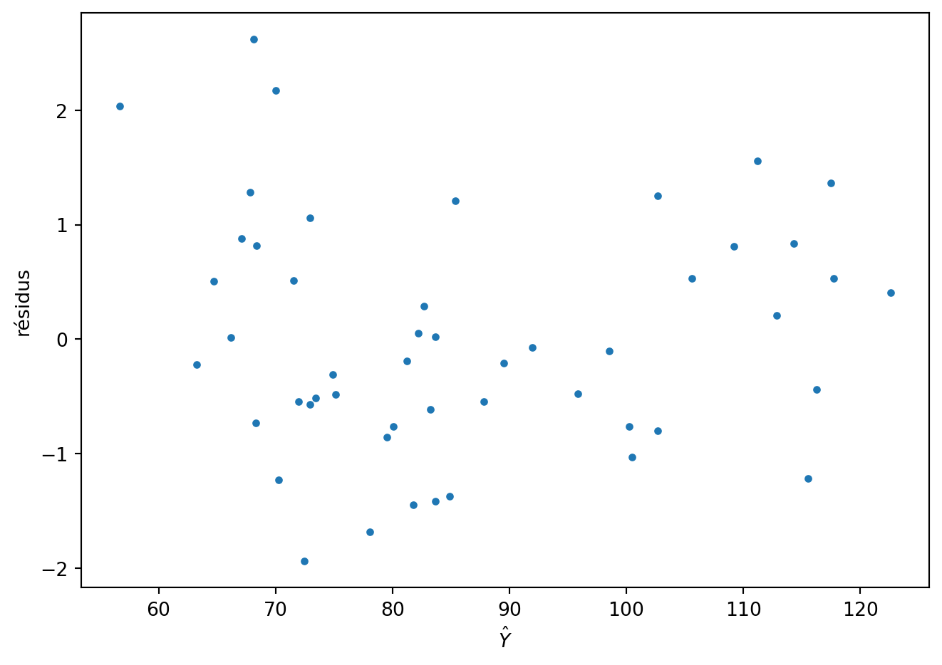

fitted2 = mod2.fittedvalues
sns.set(style="whitegrid")
fitted3 = 1/5* abs(fitted2.round(3))
dfresid = pd.concat([fitted2, pd.Series(infl.resid_studentized_external), ozone[["O3", "vent"]]], axis=1)
dfresid.columns=["residus", "ajustement", "O3", "vent"]
g = sns.FacetGrid(dfresid, col="vent")
g = g.map(plt.scatter, "ajustement", "residus")
fig.tight_layout()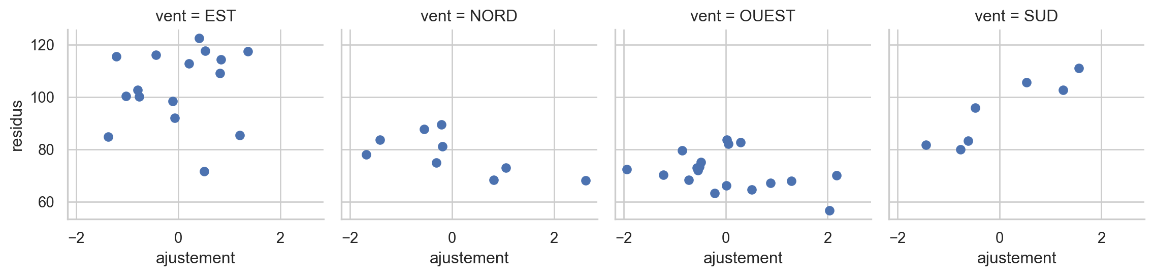

mod = smf.ols('O3 ~ vent + T12 + T12:vent', data = ozone).fit()
mod.summary()

OLS Regression Results
Dep. Variable:	O3	R-squared:	0.675
Model:	OLS	Adj. R-squared:	0.621
Method:	Least Squares	F-statistic:	12.48
Date:	Thu, 27 Mar 2025	Prob (F-statistic):	1.61e-08
Time:	16:23:51	Log-Likelihood:	-201.01
No. Observations:	50	AIC:	418.0
Df Residuals:	42	BIC:	433.3
Df Model:	7
Covariance Type:	nonrobust

	coef	std err	t	P>\|t\|	[0.025	0.975]
Intercept	45.6090	13.934	3.273	0.002	17.488	73.730
vent[T.NORD]	61.0255	31.306	1.949	0.058	-2.153	124.204
vent[T.OUEST]	19.0751	28.290	0.674	0.504	-38.017	76.168
vent[T.SUD]	-72.6691	29.975	-2.424	0.020	-133.160	-12.178
T12	2.7480	0.634	4.333	0.000	1.468	4.028
T12:vent[T.NORD]	-4.3971	1.726	-2.547	0.015	-7.881	-0.913
T12:vent[T.OUEST]	-2.4073	1.361	-1.768	0.084	-5.155	0.340
T12:vent[T.SUD]	2.6306	1.313	2.004	0.052	-0.019	5.280

Omnibus:	0.276	Durbin-Watson:	1.561
Prob(Omnibus):	0.871	Jarque-Bera (JB):	0.465
Skew:	0.007	Prob(JB):	0.793
Kurtosis:	2.528	Cond. No.	407.

Notes:
[1] Standard Errors assume that the covariance matrix of the errors is correctly specified.

La hauteur des eucalyptus

eucalypt = pd.read_csv("../donnees/eucalyptus.txt", header = 0, sep = ";")
eucalypt["bloc"] = eucalypt["bloc"].astype("category")
m_complet = smf.ols("ht ~ - 1 + bloc + bloc:circ", data = eucalypt).fit()
m_pente = smf.ols("ht ~  - 1 + bloc + circ", data = eucalypt).fit()
m_ordonne = smf.ols("ht ~ 1 + bloc:circ", data = eucalypt).fit()
sm.stats.anova_lm(m_pente, m_complet)

	df_resid	ssr	df_diff	ss_diff	F	Pr(>F)
0	1425.0	2005.895987	0.0	NaN	NaN	NaN
1	1423.0	2005.048468	2.0	0.847519	0.300746	0.740313

round(sm.stats.anova_lm(m_ordonne, m_complet),3)

	df_resid	ssr	df_diff	ss_diff	F	Pr(>F)
0	1425.0	2009.213	0.0	NaN	NaN	NaN
1	1423.0	2005.048	2.0	4.165	1.478	0.228

m_simple = smf.ols("ht ~ 1 + circ", data = eucalypt).fit()
round(sm.stats.anova_lm(m_simple,m_pente),3)

	df_resid	ssr	df_diff	ss_diff	F	Pr(>F)
0	1427.0	2052.084	0.0	NaN	NaN	NaN
1	1425.0	2005.896	2.0	46.188	16.406	0.0

plt.rc("lines", markersize=3) #
infl = m_pente.get_influence()
fig = plt.figure()
plt.plot(m_pente.fittedvalues,infl.resid_studentized_external,".")
plt.ylabel('résidus')
plt.xlabel(r'$\hat Y$')
fig.tight_layout()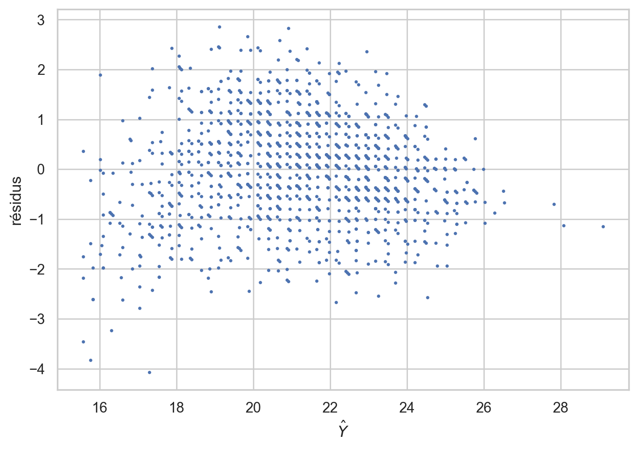

ANOVA

niveau = ozone["vent"].cat.categories
O3_parvent = []
for i in range(niveau.size):
    O3_parvent.append(list(ozone.loc[ozone["vent"]==niveau[i],"O3"]))
    
fig, ax = plt.subplots(1,1)
bplot = ax.boxplot(O3_parvent,patch_artist=True,tick_labels=niveau )
for patch in bplot["boxes"]:
     patch.set_facecolor("#5875a4")

fig.tight_layout()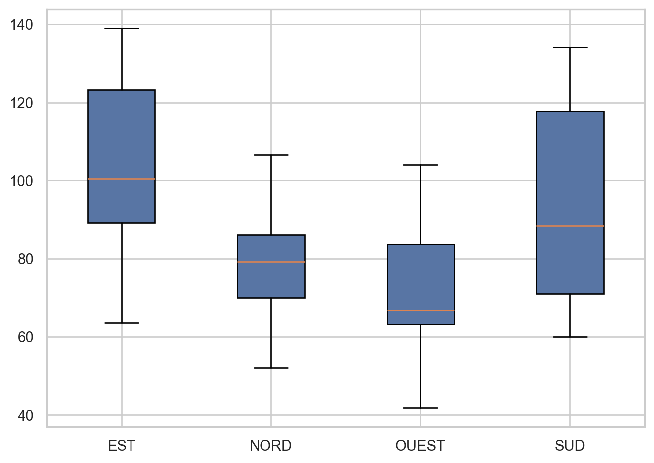

mod1 = smf.ols("O3~vent-1",data=ozone).fit()
mod1.summary()

OLS Regression Results
Dep. Variable:	O3	R-squared:	0.352
Model:	OLS	Adj. R-squared:	0.310
Method:	Least Squares	F-statistic:	8.338
Date:	Thu, 27 Mar 2025	Prob (F-statistic):	0.000156
Time:	16:23:52	Log-Likelihood:	-218.28
No. Observations:	50	AIC:	444.6
Df Residuals:	46	BIC:	452.2
Df Model:	3
Covariance Type:	nonrobust

	coef	std err	t	P>\|t\|	[0.025	0.975]
vent[EST]	103.8500	4.963	20.923	0.000	93.859	113.841
vent[NORD]	78.2889	6.618	11.830	0.000	64.968	91.610
vent[OUEST]	71.5778	4.680	15.296	0.000	62.158	80.997
vent[SUD]	94.3429	7.504	12.572	0.000	79.238	109.447

Omnibus:	1.682	Durbin-Watson:	1.737
Prob(Omnibus):	0.431	Jarque-Bera (JB):	1.184
Skew:	0.083	Prob(JB):	0.553
Kurtosis:	2.264	Cond. No.	1.60

Notes:
[1] Standard Errors assume that the covariance matrix of the errors is correctly specified.

round(sm.stats.anova_lm(mod1),3)

	df	sum_sq	mean_sq	F	PR(>F)
vent	4.0	382244.343	95561.086	242.442	0.0
Residual	46.0	18131.377	394.160	NaN	NaN

mod2 = smf.ols("O3 ~ vent", data = ozone).fit()
mod2.summary()

OLS Regression Results
Dep. Variable:	O3	R-squared:	0.352
Model:	OLS	Adj. R-squared:	0.310
Method:	Least Squares	F-statistic:	8.338
Date:	Thu, 27 Mar 2025	Prob (F-statistic):	0.000156
Time:	16:23:52	Log-Likelihood:	-218.28
No. Observations:	50	AIC:	444.6
Df Residuals:	46	BIC:	452.2
Df Model:	3
Covariance Type:	nonrobust

	coef	std err	t	P>\|t\|	[0.025	0.975]
Intercept	103.8500	4.963	20.923	0.000	93.859	113.841
vent[T.NORD]	-25.5611	8.272	-3.090	0.003	-42.212	-8.910
vent[T.OUEST]	-32.2722	6.821	-4.731	0.000	-46.003	-18.541
vent[T.SUD]	-9.5071	8.997	-1.057	0.296	-27.617	8.603

Omnibus:	1.682	Durbin-Watson:	1.737
Prob(Omnibus):	0.431	Jarque-Bera (JB):	1.184
Skew:	0.083	Prob(JB):	0.553
Kurtosis:	2.264	Cond. No.	4.51

Notes:
[1] Standard Errors assume that the covariance matrix of the errors is correctly specified.

round(sm.stats.anova_lm(mod2),3)

	df	sum_sq	mean_sq	F	PR(>F)
vent	3.0	9859.843	3286.614	8.338	0.0
Residual	46.0	18131.377	394.160	NaN	NaN

smf.ols("O3 ~ C(vent,Treatment)", data = ozone).fit().params

Intercept                      103.850000
C(vent, Treatment)[T.NORD]     -25.561111
C(vent, Treatment)[T.OUEST]    -32.272222
C(vent, Treatment)[T.SUD]       -9.507143
dtype: float64

smf.ols("O3 ~ C(vent, levels=['NORD', 'EST', 'OUEST', 'SUD'])", \
    data = ozone).fit().params

Intercept                                                   78.288889
C(vent, levels=['NORD', 'EST', 'OUEST', 'SUD'])[T.EST]      25.561111
C(vent, levels=['NORD', 'EST', 'OUEST', 'SUD'])[T.OUEST]    -6.711111
C(vent, levels=['NORD', 'EST', 'OUEST', 'SUD'])[T.SUD]      16.053968
dtype: float64

II = ozone["vent"].cat.categories.size
nI = ozone["vent"].value_counts()[ozone["vent"].cat.categories]
contr_mat = np.vstack([np.eye(II-1), (-nI[:(II-1)]).divide(nI[-1])])
contraste = ContrastMatrix(contr_mat, ["[a1]", "[a2]", "[a3]"])
mod3 = smf.ols("O3 ~ 1 + C(vent,contraste)",data=ozone).fit()
mod3.summary()

OLS Regression Results
Dep. Variable:	O3	R-squared:	0.352
Model:	OLS	Adj. R-squared:	0.310
Method:	Least Squares	F-statistic:	8.338
Date:	Thu, 27 Mar 2025	Prob (F-statistic):	0.000156
Time:	16:23:52	Log-Likelihood:	-218.28
No. Observations:	50	AIC:	444.6
Df Residuals:	46	BIC:	452.2
Df Model:	3
Covariance Type:	nonrobust

	coef	std err	t	P>\|t\|	[0.025	0.975]
Intercept	86.3000	2.808	30.737	0.000	80.648	91.952
C(vent, contraste)[a1]	17.5500	4.093	4.288	0.000	9.311	25.789
C(vent, contraste)[a2]	-8.0111	5.993	-1.337	0.188	-20.074	4.052
C(vent, contraste)[a3]	-14.7222	3.744	-3.933	0.000	-22.258	-7.187

Omnibus:	1.682	Durbin-Watson:	1.737
Prob(Omnibus):	0.431	Jarque-Bera (JB):	1.184
Skew:	0.083	Prob(JB):	0.553
Kurtosis:	2.264	Cond. No.	3.34

Notes:
[1] Standard Errors assume that the covariance matrix of the errors is correctly specified.

round(sm.stats.anova_lm(mod3),3)

	df	sum_sq	mean_sq	F	PR(>F)
C(vent, contraste)	3.0	9859.843	3286.614	8.338	0.0
Residual	46.0	18131.377	394.160	NaN	NaN

mod4 = smf.ols("O3 ~ 1+ C(vent,Sum)", data = ozone).fit()
round(sm.stats.anova_lm(mod4),3)

	df	sum_sq	mean_sq	F	PR(>F)
C(vent, Sum)	3.0	9859.843	3286.614	8.338	0.0
Residual	46.0	18131.377	394.160	NaN	NaN

print(ozone)

        Date     O3   T12   T15  Ne12  N12  S12  E12  W12     Vx    O3v  \
0   19960422   63.6  13.4  15.0     7    0    0    3    0   9.35   95.6   
1   19960429   89.6  15.0  15.7     4    3    0    0    0   5.40  100.2   
2   19960506   79.0   7.9  10.1     8    0    0    7    0  19.30  105.6   
3   19960514   81.2  13.1  11.7     7    7    0    0    0  12.60   95.2   
4   19960521   88.0  14.1  16.0     6    0    0    0    6 -20.30   82.8   
5   19960528   68.4  16.7  18.1     7    0    3    0    0  -3.69   71.4   
6   19960605  139.0  26.8  28.2     1    0    0    3    0   8.27   90.0   
7   19960612   78.2  18.4  20.7     7    4    0    0    0   4.93   60.0   
8   19960619  113.8  27.2  27.7     6    0    4    0    0  -4.93  125.8   
9   19960627   41.8  20.6  19.7     8    0    0    0    1  -3.38   62.6   
10  19960704   65.0  21.0  21.1     6    0    0    0    7 -23.68   38.0   
11  19960711   73.0  17.4  22.8     8    0    0    0    2  -6.24   70.8   
12  19960719  126.2  26.9  29.5     2    0    0    4    0  14.18  119.8   
13  19960726  127.8  25.5  27.8     3    0    0    5    0  13.79  103.6   
14  19960802   61.6  19.4  21.5     7    6    0    0    0  -7.39   69.2   
15  19960810   63.6  20.8  21.4     7    0    0    0    5 -13.79   48.0   
16  19960817  134.2  29.5  30.6     2    0    3    0    0   1.88  118.6   
17  19960824   67.2  21.7  20.3     7    0    0    0    7 -24.82   60.0   
18  19960901   87.8  19.7  21.7     5    0    0    3    0   9.35   74.4   
19  19960908   96.8  19.0  21.0     6    0    0    8    0  28.36  103.8   
20  19960915   89.6  20.7  22.9     1    0    0    4    0  12.47   78.8   
21  19960923   66.4  18.0  18.5     7    0    0    0    2  -5.52   72.2   
22  19960930   60.0  17.4  16.4     8    0    6    0    0 -10.80   53.4   
23  19970414   90.8  16.3  18.1     0    0    0    5    0  18.00   89.0   
24  19970422  104.2  13.6  14.4     1    0    0    1    0   3.55   97.8   
25  19970429   70.0  15.8  16.7     7    7    0    0    0 -12.60   61.4   
26  19970708   96.2  26.0  27.3     2    0    0    5    0  16.91   87.4   
27  19970715   65.6  23.5  23.7     7    0    0    0    3  -9.35   67.8   
28  19970722  109.2  26.3  27.3     4    0    0    5    0  16.91   98.6   
29  19970730   86.2  21.8  23.6     6    4    0    0    0   2.50  112.0   
30  19970806   87.4  24.8  26.6     3    0    0    0    2  -7.09   49.8   
31  19970813   84.0  25.2  27.5     3    0    0    0    3 -10.15  131.8   
32  19970821   83.0  24.6  27.9     3    0    0    0    2  -5.52  113.8   
33  19970828   59.6  16.8  19.0     7    0    0    0    8 -27.06   55.8   
34  19970904   52.0  17.1  18.3     8    5    0    0    0  -3.13   65.8   
35  19970912   73.8  18.0  18.3     7    0    5    0    0 -11.57   90.4   
36  19970919  129.0  28.9  30.0     1    0    0    3    0   8.27  111.4   
37  19970926  122.4  23.4  25.4     0    0    0    2    0   5.52  118.6   
38  19980504  106.6  13.0  14.3     3    7    0    0    0  12.60   84.0   
39  19980511  121.8  26.0  28.0     2    0    4    0    0   2.50  109.8   
40  19980518  116.2  24.9  25.8     2    0    0    5    0  18.00  142.8   
41  19980526   81.4  18.4  16.8     7    0    0    0    4 -14.40   80.8   
42  19980602   88.6  18.7  19.6     5    0    0    0    5 -15.59   60.4   
43  19980609   63.0  20.4  16.6     7    0    0    0    8 -22.06   79.8   
44  19980617  104.0  19.6  21.2     6    0    0    0    3 -10.80   84.6   
45  19980624   88.4  23.2  23.9     4    0    4    0    0  -7.20   92.6   
46  19980701   83.8  19.8  20.3     8    0    0    5    0  17.73   40.2   
47  19980709   56.4  18.9  19.3     8    0    0    0    4 -14.40   73.6   
48  19980716   50.4  19.7  19.3     7    0    0    0    5 -17.73   59.0   
49  19980724   79.2  21.1  21.9     3    4    0    0    0   9.26   55.2   

      nebu   vent  
0    NUAGE    EST  
1   SOLEIL   NORD  
2    NUAGE    EST  
3    NUAGE   NORD  
4    NUAGE  OUEST  
5    NUAGE    SUD  
6   SOLEIL    EST  
7    NUAGE   NORD  
8    NUAGE    SUD  
9    NUAGE  OUEST  
10   NUAGE  OUEST  
11   NUAGE  OUEST  
12  SOLEIL    EST  
13  SOLEIL    EST  
14   NUAGE   NORD  
15   NUAGE  OUEST  
16  SOLEIL    SUD  
17   NUAGE  OUEST  
18  SOLEIL    EST  
19   NUAGE    EST  
20  SOLEIL    EST  
21   NUAGE  OUEST  
22   NUAGE    SUD  
23  SOLEIL    EST  
24  SOLEIL    EST  
25   NUAGE   NORD  
26  SOLEIL    EST  
27   NUAGE  OUEST  
28  SOLEIL    EST  
29   NUAGE   NORD  
30  SOLEIL  OUEST  
31  SOLEIL  OUEST  
32  SOLEIL  OUEST  
33   NUAGE  OUEST  
34   NUAGE   NORD  
35   NUAGE    SUD  
36  SOLEIL    EST  
37  SOLEIL    EST  
38  SOLEIL   NORD  
39  SOLEIL    SUD  
40  SOLEIL    EST  
41   NUAGE  OUEST  
42  SOLEIL  OUEST  
43   NUAGE  OUEST  
44   NUAGE  OUEST  
45  SOLEIL    SUD  
46   NUAGE    EST  
47   NUAGE  OUEST  
48   NUAGE  OUEST  
49  SOLEIL   NORD

ozone = pd.read_csv("../donnees/ozone.txt", header = 0, sep = ";")
ozone["vent"]=ozone["vent"].astype("category")
ozone["nebu"]=ozone["nebu"].astype("category")
plt.rcParams['font.size'] = '7'
from statsmodels.graphics.api import interaction_plot
cc2 = cm.Set1(range(ozone["vent"].cat.categories.size))
fig, axs = plt.subplots(1,2)
plt.rcParams['font.size'] = '4'
interaction_plot(ozone["vent"].astype("str"), ozone["nebu"].astype("str"), ozone["O3"], colors=cc2[:2], markers=['^','D'],ax=axs[0])
interaction_plot( ozone["nebu"].astype("str"), ozone["vent"].astype("str"),ozone["O3"], colors=cc2, markers=['^','D',"*","8"],ax=axs[1])
fig.tight_layout()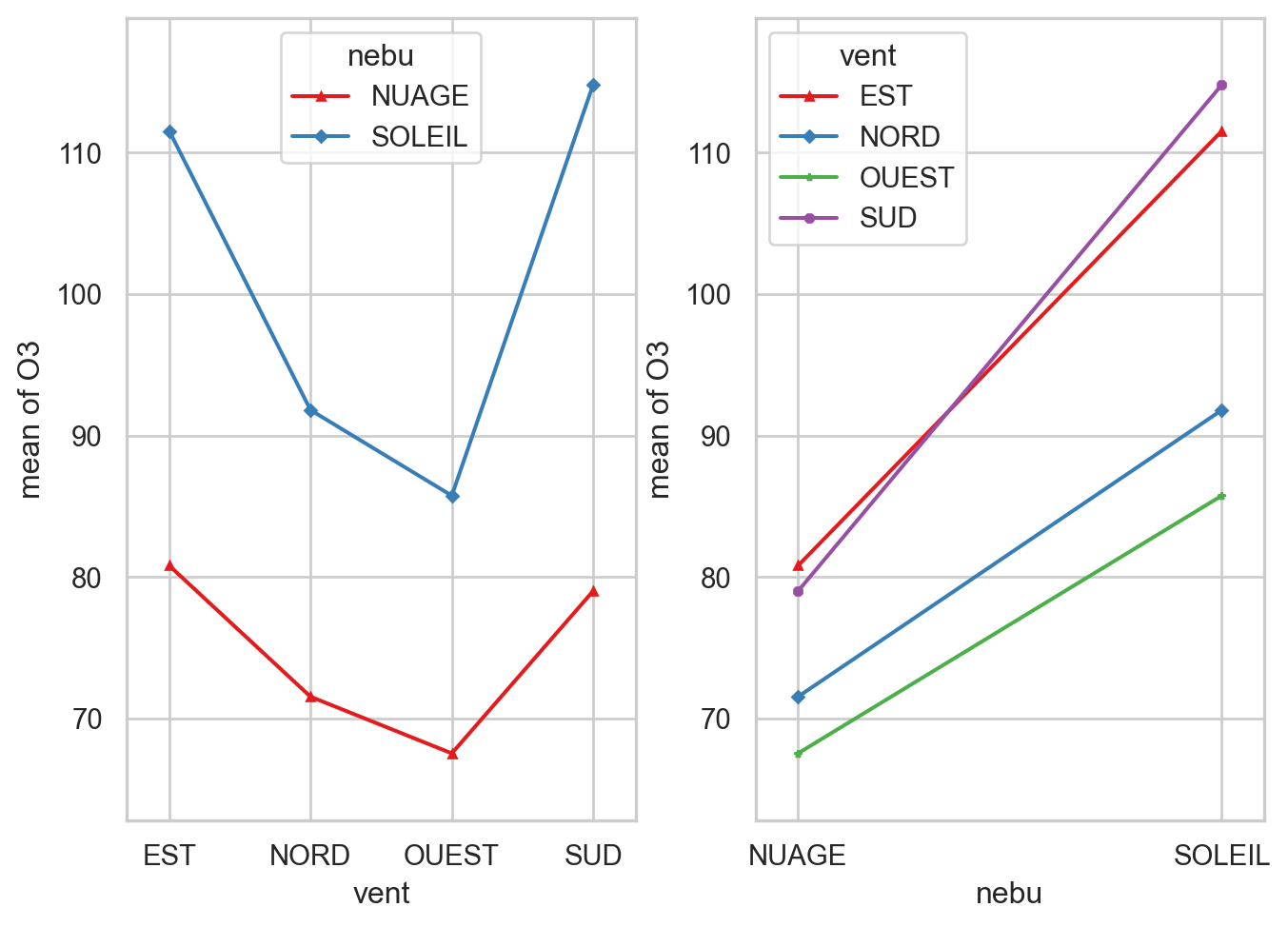

mod1 = smf.ols("O3 ~ vent + nebu + vent:nebu", data = ozone).fit()
mod2 = smf.ols("O3 ~ vent + nebu ", data = ozone).fit()
sm.stats.anova_lm(mod2,mod1)

	df_resid	ssr	df_diff	ss_diff	F	Pr(>F)
0	45.0	11729.859077	0.0	NaN	NaN	NaN
1	42.0	11246.238571	3.0	483.620506	0.60204	0.617302

mod3 = smf.ols("O3 ~ vent", data = ozone).fit()
round(sm.stats.anova_lm(mod3,mod2),3)

	df_resid	ssr	df_diff	ss_diff	F	Pr(>F)
0	46.0	18131.377	0.0	NaN	NaN	NaN
1	45.0	11729.859	1.0	6401.518	24.559	0.0

round(sm.stats.anova_lm(mod3, mod2, mod1),3)

	df_resid	ssr	df_diff	ss_diff	F	Pr(>F)
0	46.0	18131.377	0.0	NaN	NaN	NaN
1	45.0	11729.859	1.0	6401.518	23.907	0.000
2	42.0	11246.239	3.0	483.621	0.602	0.617

round(sm.stats.anova_lm(mod1),3)

	df	sum_sq	mean_sq	F	PR(>F)
vent	3.0	9859.843	3286.614	12.274	0.000
nebu	1.0	6401.518	6401.518	23.907	0.000
vent:nebu	3.0	483.621	161.207	0.602	0.617
Residual	42.0	11246.239	267.768	NaN	NaN

Retour au sommet