import pandas as pd; import numpy as np
import matplotlib.pyplot as plt
import scipy as sp
from scipy import stats
import statsmodels.formula.api as smf
import statsmodels.api as sm
import statsmodels.regression.linear_model as smlm
import sys
sys.path.append('../modules')
import choixglmstats13 Régression de Poisson
Le modèle linéaire généralisé
Exemple : modélisation du nombre de visites
Malaria = pd.read_csv("../donnees/poissonData3.csv", header=0, sep=',')
Malaria["Sexe"] = Malaria["Sexe"].astype("category")
Malaria["Prev"] = Malaria["Prev"].astype("category")
print(Malaria.describe())
Age Altitude Duree Nmalaria
count 1627.000000 1522.000000 1627.000000 1627.000000
mean 419.359557 1294.714389 619.263061 4.687154
std 247.929838 44.198415 420.990175 4.153109
min 10.000000 1129.000000 0.000000 0.000000
25% 220.000000 1266.000000 172.000000 1.000000
50% 361.000000 1298.000000 721.000000 4.000000
75% 555.000000 1320.000000 1011.000000 7.000000
max 1499.000000 1515.000000 1464.000000 26.000000print(Malaria.isna().sum(axis=0))Sexe 0
Age 0
Altitude 105
Prev 0
Duree 0
Nmalaria 0
dtype: int64Malaria = Malaria[["Sexe","Prev","Duree","Nmalaria"]]
plt.plot(Malaria.Duree, Malaria.Nmalaria, 'o')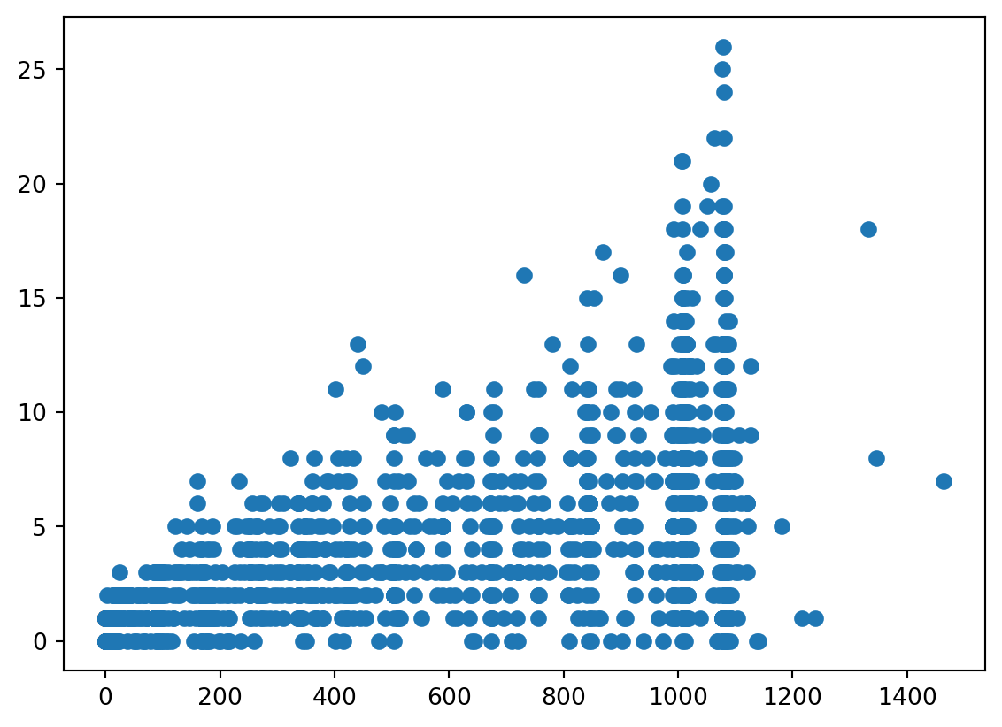
fig = plt.figure()
modele = smf.ols("Nmalaria ~ 1+ Duree", data = Malaria).fit()
plt.plot(Malaria.Duree, Malaria.Nmalaria, 'o')
grille = pd.DataFrame({'Duree': np.linspace(Malaria.Duree.min(), Malaria.Duree.max(), 2)})
calcprev = modele.get_prediction(grille)
plt.plot(Malaria.Duree, Malaria.Nmalaria, 'o', grille.Duree,  calcprev.predicted_mean, '-')
fig.tight_layout()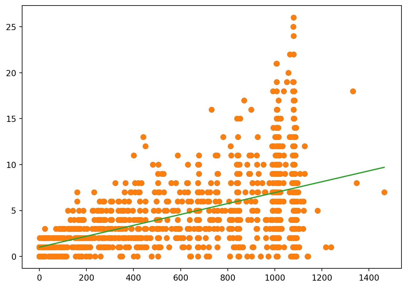
modP = smf.glm("Nmalaria ~ 1+ Duree", data = Malaria, family=sm.families.Poisson()).fit()
modP.summary()| Dep. Variable: | Nmalaria | No. Observations: | 1627 |
| Model: | GLM | Df Residuals: | 1625 |
| Model Family: | Poisson | Df Model: | 1 |
| Link Function: | Log | Scale: | 1.0000 |
| Method: | IRLS | Log-Likelihood: | -4060.3 |
| Date: | Tue, 04 Feb 2025 | Deviance: | 3325.2 |
| Time: | 14:27:57 | Pearson chi2: | 3.17e+03 |
| No. Iterations: | 5 | Pseudo R-squ. (CS): | 0.7691 |
| Covariance Type: | nonrobust |
| coef | std err | z | P>|z| | [0.025 | 0.975] | |
| Intercept | 0.4295 | 0.031 | 13.853 | 0.000 | 0.369 | 0.490 |
| Duree | 0.0015 | 3.42e-05 | 44.144 | 0.000 | 0.001 | 0.002 |
fig = plt.figure()
plt.plot(Malaria.Duree, Malaria.Nmalaria, 'o')
grille2 = pd.DataFrame({'Duree': np.linspace(Malaria.Duree.min(), Malaria.Duree.max(), 1500)})
calcprev2 = modP.get_prediction(grille2)
plt.plot(Malaria.Duree, Malaria.Nmalaria, 'o', grille.Duree,  calcprev.predicted_mean, '-', grille2.Duree,  calcprev2.predicted_mean, '--')
fig.tight_layout()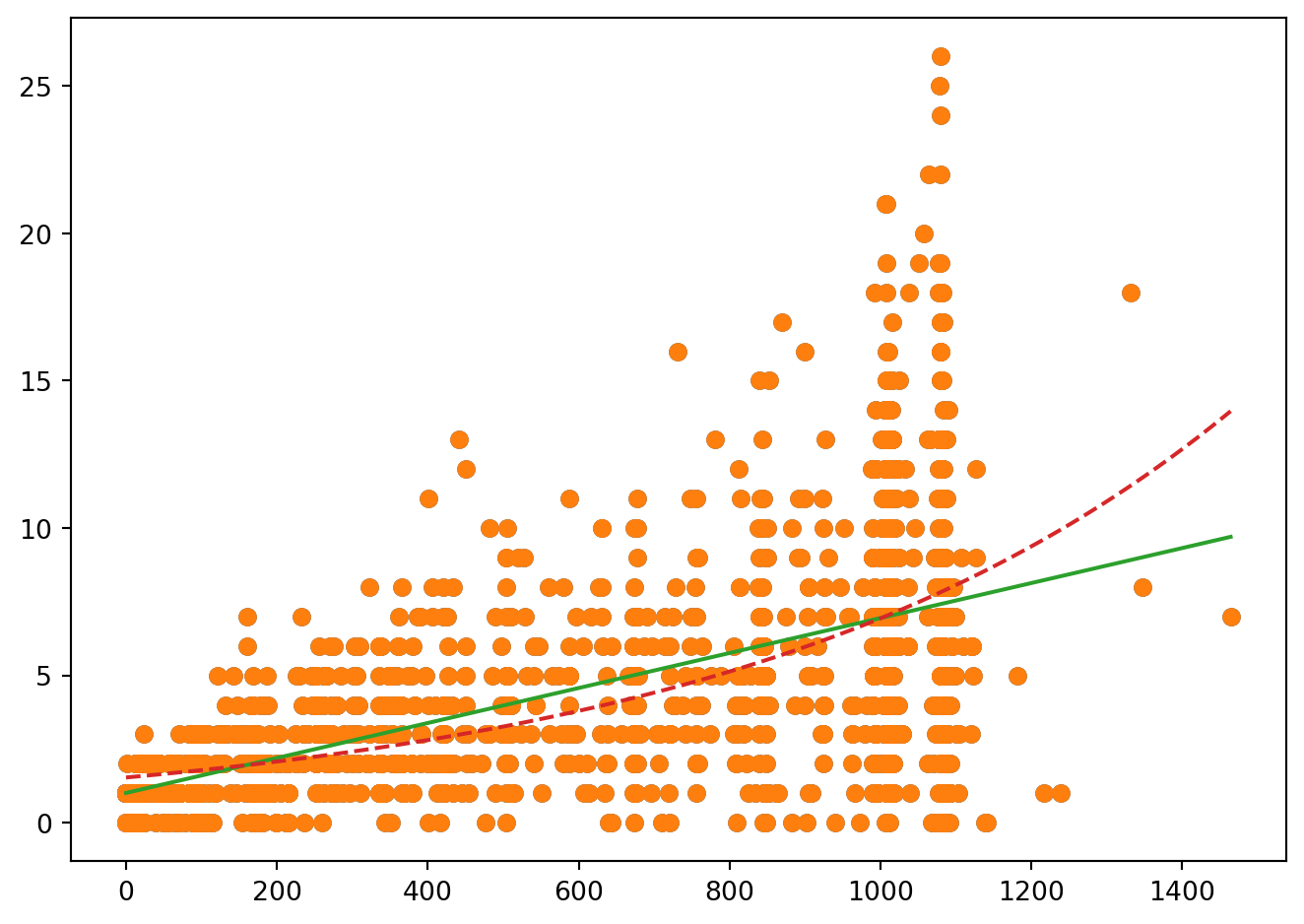
Régression log-linéaire
modP3 = smf.glm("Nmalaria ~ 1+ Duree + Sexe + Prev", data = Malaria, family=sm.families.Poisson()).fit()
print(modP3.summary())
Generalized Linear Model Regression Results
==============================================================================
Dep. Variable: Nmalaria No. Observations: 1627
Model: GLM Df Residuals: 1621
Model Family: Poisson Df Model: 5
Link Function: Log Scale: 1.0000
Method: IRLS Log-Likelihood: -4056.3
Date: Tue, 04 Feb 2025 Deviance: 3317.3
Time: 14:27:57 Pearson chi2: 3.17e+03
No. Iterations: 5 Pseudo R-squ. (CS): 0.7703
Covariance Type: nonrobust
===========================================================================================
coef std err z P>|z| [0.025 0.975]
-------------------------------------------------------------------------------------------
Intercept 0.1623 0.180 0.900 0.368 -0.191 0.516
Sexe[T.M] 0.0551 0.023 2.398 0.016 0.010 0.100
Prev[T.Moustiquaire] 0.2433 0.177 1.371 0.170 -0.105 0.591
Prev[T.Rien] 0.2256 0.178 1.266 0.205 -0.124 0.575
Prev[T.Serpentin/Spray] 0.2452 0.185 1.324 0.185 -0.118 0.608
Duree 0.0015 3.43e-05 44.031 0.000 0.001 0.002
===========================================================================================mod3= smf.glm("Nmalaria ~ 1+ Duree + Sexe + C(Prev, Treatment('Rien'))", data = Malaria, family=sm.families.Poisson()).fit()
print(mod3.summary()) Generalized Linear Model Regression Results
==============================================================================
Dep. Variable: Nmalaria No. Observations: 1627
Model: GLM Df Residuals: 1621
Model Family: Poisson Df Model: 5
Link Function: Log Scale: 1.0000
Method: IRLS Log-Likelihood: -4056.3
Date: Tue, 04 Feb 2025 Deviance: 3317.3
Time: 14:27:57 Pearson chi2: 3.17e+03
No. Iterations: 5 Pseudo R-squ. (CS): 0.7703
Covariance Type: nonrobust
=================================================================================================================
coef std err z P>|z| [0.025 0.975]
-----------------------------------------------------------------------------------------------------------------
Intercept 0.3879 0.039 9.951 0.000 0.311 0.464
Sexe[T.M] 0.0551 0.023 2.398 0.016 0.010 0.100
C(Prev, Treatment('Rien'))[T.Autre] -0.2256 0.178 -1.266 0.205 -0.575 0.124
C(Prev, Treatment('Rien'))[T.Moustiquaire] 0.0177 0.026 0.691 0.490 -0.032 0.068
C(Prev, Treatment('Rien'))[T.Serpentin/Spray] 0.0196 0.059 0.333 0.739 -0.096 0.135
Duree 0.0015 3.43e-05 44.031 0.000 0.001 0.002
=================================================================================================================modP2= smf.glm("Nmalaria ~ 1+ Duree + Sexe ", data = Malaria, family=sm.families.Poisson()).fit()smlm.RegressionResults.compare_lr_test(modP3,modP2)(2.4488233421689074, 0.4846108842015914, 3)sp.stats.chi2.ppf(0.95,3)7.814727903251179print(modP3.conf_int(alpha=0.05)) 0 1
Intercept -0.191170 0.515791
Sexe[T.M] 0.010071 0.100107
Prev[T.Moustiquaire] -0.104566 0.591101
Prev[T.Rien] -0.123561 0.574727
Prev[T.Serpentin/Spray] -0.117722 0.608171
Duree 0.001443 0.001577Malaria = pd.read_csv("../donnees/poissonData.csv", header=0, sep=",")
Malaria.dropna(axis=0, inplace=True)form ="Nmalaria ~ " + "+".join(Malaria.columns[ :-1 ])
mod_sel = choixglmstats.bestglm(Malaria, upper=form, family=sm.families.Poisson())print(mod_sel.sort_values(by=["BIC","nb_var"]).iloc[:3,[1,3]]) var_added BIC
13 (Altitude, Duree, Age) 7392.274194
20 (Altitude, Duree) 7395.141592
2 (Sexe, Altitude, Duree, Age) 7397.380825print(mod_sel.sort_values(by=["AIC","nb_var"]).iloc[:3,[1,2]]) var_added AIC
2 (Sexe, Altitude, Duree, Age) 7370.741923
13 (Altitude, Duree, Age) 7370.963072
0 (Sexe, Altitude, Duree, Prev, Age) 7374.648450