10 Régression sur composantes : PCR et PLS

import pandas as pd; import numpy as np
import matplotlib.pyplot as plt
import statsmodels.formula.api as smf
from sklearn.preprocessing import StandardScaler
from sklearn.decomposition import PCA
from sklearn.linear_model import LinearRegression
from sklearn.cross_decomposition import PLSRegression
from sklearn.pipeline import Pipeline
from sklearn.model_selection import GridSearchCV, KFold
from sklearn.metrics import mean_squared_error
import sys
sys.path.append('../modules')
from ols_step_sk import LinearRegressionSelectionFeatureIC

Régression sur composantes principales (PCR)

ozone = pd.read_csv("../donnees/ozone.txt", header = 0, sep = ";", index_col=0).iloc[:,:10]
X = ozone.iloc[:,1:10]
y = ozone.iloc[:,:1]
reg = smf.ols('O3 ~ T12 + T15 + Ne12 + N12 + S12 + E12 + W12 + Vx + O3v', data=ozone).fit()
reg.summary()

OLS Regression Results
Dep. Variable:	O3	R-squared:	0.751
Model:	OLS	Adj. R-squared:	0.694
Method:	Least Squares	F-statistic:	13.37
Date:	Fri, 31 Jan 2025	Prob (F-statistic):	1.51e-09
Time:	17:30:32	Log-Likelihood:	-194.43
No. Observations:	50	AIC:	408.9
Df Residuals:	40	BIC:	428.0
Df Model:	9
Covariance Type:	nonrobust

	coef	std err	t	P>\|t\|	[0.025	0.975]
Intercept	54.7278	17.279	3.167	0.003	19.806	89.650
T12	-0.3518	1.573	-0.224	0.824	-3.531	2.827
T15	1.4972	1.538	0.974	0.336	-1.611	4.605
Ne12	-4.1922	1.064	-3.941	0.000	-6.342	-2.042
N12	1.2755	1.363	0.936	0.355	-1.480	4.031
S12	3.1711	1.911	1.660	0.105	-0.691	7.033
E12	0.5277	1.943	0.272	0.787	-3.399	4.454
W12	2.4749	2.072	1.194	0.239	-1.713	6.663
Vx	0.6077	0.486	1.251	0.218	-0.374	1.589
O3v	0.2454	0.096	2.543	0.015	0.050	0.440

Omnibus:	0.252	Durbin-Watson:	1.887
Prob(Omnibus):	0.881	Jarque-Bera (JB):	0.364
Skew:	0.153	Prob(JB):	0.833
Kurtosis:	2.716	Cond. No.	859.

Notes:
[1] Standard Errors assume that the covariance matrix of the errors is correctly specified.

mod_lin9v = LinearRegression()
mod_lin9v.fit(X,y)
np.round(mod_lin9v.coef_,2)

array([[-0.35,  1.5 , -4.19,  1.28,  3.17,  0.53,  2.47,  0.61,  0.25]])

reg_bic = LinearRegressionSelectionFeatureIC(crit="bic")
reg_bic.fit(X, y)
X.columns[reg_bic.selected_features_]

Index(['T15', 'Ne12', 'Vx', 'O3v'], dtype='object')

cr = StandardScaler()
acp = PCA(n_components=9)
pipe_acp = Pipeline(steps=[("cr", cr), ("acp", acp)])
pipe_acp.fit(X)
Xortho = pipe_acp.fit_transform(X)
reg_bic.fit(Xortho, y)
varsel = reg_bic.selected_features_
varsel

[0, 4]

step_cr = pipe_acp.named_steps["cr"]
stdX = step_cr.scale_
meanX = step_cr.mean_
coef_pcr =reg_bic.coef_
step_acp = pipe_acp.named_steps["acp"]
P = step_acp.components_[reg_bic.selected_features_,]
betafinpcr = P.T.dot(coef_pcr.T)[:,0]/stdX
intercept = y.mean(axis=0) - meanX.dot(betafinpcr.T)
np.round(np.append(intercept, betafinpcr),2)

array([ 5.279e+01,  4.100e-01,  4.700e-01, -2.540e+00, -8.700e-01,
        2.000e-02,  1.060e+00, -8.500e-01,  2.300e-01,  3.400e-01])

cr = StandardScaler()
acp = PCA()
reg = LinearRegression()
pipe_pcr = Pipeline(steps=[("cr", cr), ("acp", acp), ("reg", reg)])
param_grid_pcr = { "acp__n_components" : list(range(1,10))}
kf = KFold(n_splits=4, shuffle=True, random_state=0)
cv_pcr = GridSearchCV(pipe_pcr, param_grid_pcr, cv=kf, scoring = 'neg_mean_squared_error', n_jobs=3).fit(X, y)

import matplotlib.cm as cm
colors = cm.Set1(range(1))
colors2 = colors
colors2[:,3] = colors2[:,3] -0.7
fig, ax1 = plt.subplots(1, 1)
ax1.errorbar(list(range(1,10)), -cv_pcr.cv_results_["mean_test_score"],
             cv_pcr.cv_results_["std_test_score"]/kf.n_splits**0.5 , capsize=10,  c=colors[0], ecolor=colors2[0])
fig.tight_layout()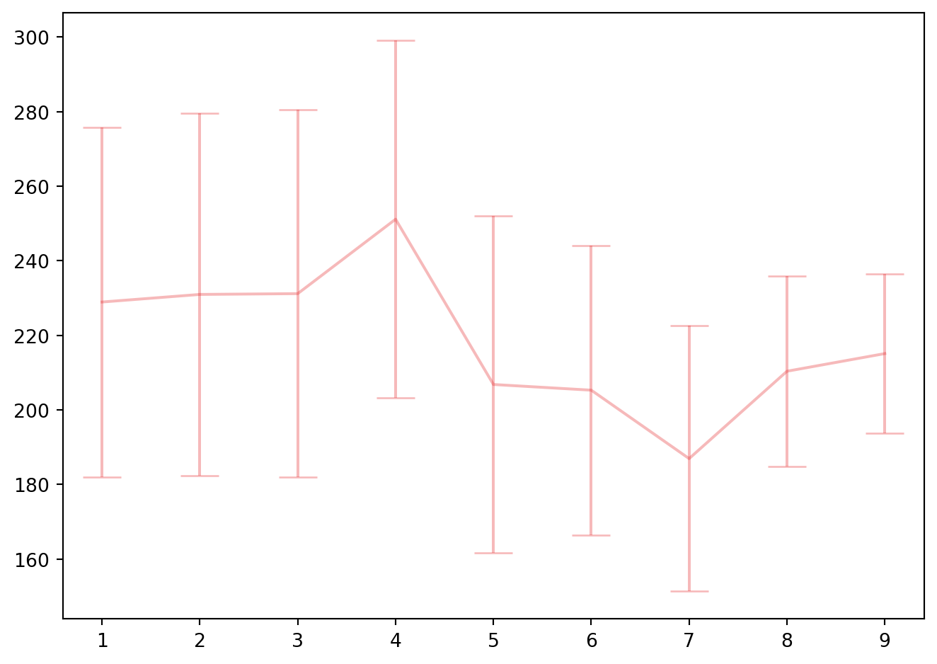

bestpcr =  cv_pcr.best_estimator_
cv_pcr.best_params_
step_reg = bestpcr.named_steps["reg"]
coef_pcr = step_reg.coef_
step_cr =  bestpcr.named_steps["cr"]
stdX = step_cr.scale_
meanX = step_cr.mean_
step_acp = bestpcr.named_steps["acp"]
P = step_acp.components_
betafinpcr = P.T.dot(coef_pcr.T)[:,0]/stdX
intercept = y.mean(axis=0) - meanX.dot(betafinpcr.T)
np.round(np.append(intercept, betafinpcr),2)

array([58.33,  0.68,  0.44, -4.45,  1.24,  2.11,  1.84,  0.6 ,  0.15,
        0.25])

Régression aux moindres carrés partiels (PLS)

regpls = PLSRegression()
param_grid_pls = { "n_components" : list(range(1,10))}
kf = KFold(n_splits=4, shuffle=True, random_state=0)
cv_pls = GridSearchCV(regpls, param_grid_pls, cv=kf, scoring = 'neg_mean_squared_error').fit(X, y)

colors = cm.Set1(range(1))
colors2 = colors
colors2[:,3] = colors2[:,3] -0.6
fig, ax1 = plt.subplots(1, 1)
ax1.errorbar(list(range(1,10)), -cv_pls.cv_results_["mean_test_score"],  cv_pls.cv_results_["std_test_score"]/kf.n_splits**0.5 ,  capsize=10, c=colors[0], ecolor=colors2[0])
fig.tight_layout()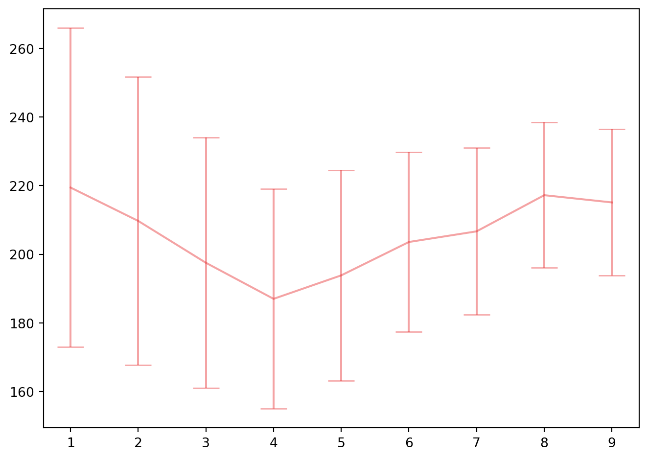

bestpls =  cv_pls.best_estimator_
cv_pls.best_params_
bestpls.fit(X,y)
bestpls.coef_

array([[ 0.41610174,  0.53217084, -4.4244714 ,  0.37042358,  1.60857405,
         0.98429296,  0.56053927,  0.24800203,  0.26473814]])

scalerX = StandardScaler().fit(X)
stdX = scalerX.scale_
meanX = scalerX.mean_
betafinpls = bestpls.coef_[:,0]/stdX
intercept = y.mean(axis=0) - meanX.dot(betafinpls.T)
np.append(intercept, betafinpls)

array([7.95723726e+01, 8.99163083e-02, 8.43936432e-02, 1.65784166e-01,
       1.98000066e-01, 2.80306490e-01, 1.88545955e-01, 1.71475028e-01,
       3.09237815e-02, 1.68441318e-02])

Retour au sommet